Chris Helzer is Director of Science and Stewardship for The Nature Conservancy in Nebraska, where he conducts research and supervises the Conservancy’s preserve stewardship program. He also helps develop, test, and share prairie management and restoration strategies.
Chris is also dedicated to raising awareness about the value of prairies through his photography, writing and presentations. He is the author of The Prairie Ecologist blog, and two books: The Ecology and Management of Prairies and Hidden Prairie: Photographing Life in One Square Meter. He is also a frequent contributor to NEBRASKAland magazine and other publications. Chris and his family live in Aurora, Nebraska.
As a prairie ecologist who tries to help others fall in love with prairies, one of the primary obstacles I run into is that most people can’t recognize very many of the incredible species that live in grasslands. If one plant or animal looks just like another, everything looks the same! As a result, when those people visit a prairie for the first time, it appears to be a flat, boring wasteland – a monochromatic smear of vegetation and bugs. That’s uninteresting, unattractive, and uninviting. It’s also a huge problem for conservation since we need people to care enough to support our work.
As a response to this crisis, I’ve decided to start a new periodic series of blog posts aimed at helping people distinguish between some of the more common groups of prairie species they might encounter. This is not a field guide and won’t (usually) help people identify individual species. Instead, the purpose is simply to provide some very basic tips that will help them tell some organisms apart from others and start to see some of the diversity those of us familiar with prairies sometimes take for granted.
For this inaugural installment, I’ll start with two common groups of animals: butterflies and grasshoppers. Those of us who see these animals frequently can easily tell one from the other but probably don’t think much about how we’re doing it. For the uninitiated, the two can look very similar.
ButterflyGrasshopper
It’s easy to see how these two organisms can be difficult to distinguish from each other. Both have long bodies, large eyes, six legs, and antennae, and those are just a few of their similarities! There are some stark differences too, but it’s important to know which are consistent, and thus useful.
For example, when looking at the above photos, you might immediately think, “Oh, that’s easy! Grasshoppers and green and butterflies are multi-colored!” I implore you not to fall into that trap. Both grasshoppers and butterflies can come in a wide variety of colors and color combinations, making color completely unreliable as a way to separate them. However, there are a few key characteristics than can help you tell them apart. We’ll start with the most helpful…
Tongue
If you look closely at a butterfly, you may be able to see the long curling tongue it uses to access nectar from deep inside a flower. When it is feeding, this tongue is often extended in a way that makes it relatively easy to spot. Grasshoppers, on the other hand, don’t have a tongue. Instead, they have various other anatomical features that fill some of the roles of a tongue, but come with complicated names like “hypopharynx” or “three-segmented labial palps”.
The circled structure in this butterfly photo is the tongue, which you can see it using to extract nectar from this flower.Grasshoppers have no tongue. Instead, they have complex, confusing-looking mouthparts designed to bite and chew plant matter.
Since butterflies have long tongues and grasshoppers have no tongues, this is obviously a great first step toward separating the two animals from each other. When you see an insect and you’re not immediately sure whether it is a butterfly or grasshopper, look first for the tell-tale tongue. It’s even alliterative!
Spines on legs
Unfortunately, it’s not always possible to use the presence or absence of a tongue to tell a grasshopper from a butterfly. Sometimes, butterflies either don’t have their tongue extended or it is out of sight because of the way the butterfly is positioned. This is problematic, but not a complete catastrophe. If you can’t see the tongue but aren’t completely sure you’re looking at a grasshopper, look next at the legs.
As you can see in this photo, the place where this creature’s tongue might be is obscured by the petal of whatever kind of plant that is. This unusual situation makes it necessary to have more than one characteristic to rely on when trying to decide if it’s a butterfly or grasshopper.
Most grasshoppers have spines on their legs. No one knows why this is, but it can be helpful when trying to distinguish between grasshoppers and butterflies since butterflies have hairy legs but almost never spiny legs.
The front legs of a grasshopper may or may not have obvious spines. Some do, but others merely have hairs like those seen on butterfly legs. However, if you focus on the rear legs (the big ones), grasshoppers almost always display prominent spines, especially on the leg segment closest to their feet.
There’s a simple rhyming phrase than can help you remember this clue. It’s easy to imagine the spines on a grasshopper’s leg as being able to pop a balloon. Thus, you can remember that grasshoppers have spiny legs with the phrase, “Grasshoppers are balloon poppers”. Easy peasy!
The spines on the lower segment of this grasshopper’s leg clearly distinguishes it from a butterfly. That’s particular helpful in this case because its mouth is partially obscured by one of its front legs, making it difficult to tell if it has a tongue.
Used in tandem with each other, the combination of tongues and leg spines will usually be sufficient to tell whether a particular insect is a grasshopper or a butterfly. In desperate situations, however, there is one final feature that can be used…
Bulbous antennae tips
While the tongue or leg spines of these creatures can (rarely) be simultaneously concealed, the antennae will almost always be visible in those cases. For example, if you look back at the earlier photo of the orange creature in which the tongue wasn’t visible, you’ll notice that the legs are also concealed. Vexing! But look closer, and you’ll see that the antennae are clearly visible. This saving grace will allow us to decide with confidence whether it is a butterfly or grasshopper.
Antennae are the two linear projections protruding from the heads of both grasshoppers and butterflies. These likely serve a purpose that science will someday discover. Initially, you might think the fact that both creatures have antennae would make those structures unhelpful in telling one creature from another. Look more closely, however, and you’ll notice that butterflies have little knobs or bulbs at the extreme tips of their antennae. The antennae of grasshoppers do not have this feature.
In this photo, both the tongue and legs are difficult to see, but the circled portion of the antennae clearly shows a swelling, or thickening of the structure. Thus, we can safely conclude that it’s a butterfly.
There’s a fun and easy way to remember the significance of the bulbous tip of a butterfly’s antennae. The term ‘grasshopper’ implies a creature that can jump, right? Whether or not that’s true isn’t important. What matters is the following phrase: “If it has a bump, it probably can’t jump.” In other words, a creature with a ‘bump’ on the tip of its antennae isn’t a grasshopper.
You’ve now learned three different cues you can employ to tell whether an animal is a butterfly or a grasshopper. First, look for a tongue. Second, try to see whether there are spines on the legs (especially the hind legs). Third, check the antennae to see if they have a swollen tip. Any one of these may be enough to make an identification, but two or more are firmly diagnostic.
Let’s test your knowledge by looking again at a photo shown earlier.
Can you tell if this is a grasshopper or butterfly?
Only one of the three key characteristics is visible in the above photo. Can you tell whether it is a butterfly or grasshopper?
It is, of course, a butterfly because “if it has a bump, it probably can’t jump”. Well done!
I hope this has been a helpful guide for telling the difference between butterflies and grasshoppers. If you did find it useful, please share it with your friends and family – then stay tuned for future installments of this series and learn about other fascinating and beautiful prairie plants and animals!
Quick reminder: Applications for the J.E. Weaver grants ($1500) for graduate students working on conservation topics related to the Great Plains are due March 3, 2023. Information can be found here.
This one’s for the real prairie nerds out there. It’s long, full of data, and will probably appeal mostly to people who restore prairies or study prairie restoration. Apologies to those of you who mainly follow this blog for the pretty photos…
Despite the obscene number of graphs, I do think there’s a pretty fascinating story here. I’ll do my best to tell it in a compelling way. The story starts with the pattern with which a brand new prairie plant community assembles itself. That’s a good tale in itself, but then I compare that pattern to two other nearby plantings with surprising (to me) results. Finally, the significant role of land stewardship and its impact on establishment fills the third and final chapter of the story.
Silky prairie clover (Dalea villosa) and Junegrass (Koeleria macrantha) in the Derr Pivot sandhills restoration (July 2014 photo).
First, the basic information:
The 100 acre Derr Pivot prairie restoration was planted into a former soybean field in the fall of 2001. We call it a 2002 restoration because 2002 was its first growing season. The site is located in some sandy hills south of the river at The Nature Conservancy’s Platte River Prairies. Seed for the project was locally-harvested and the seed mix included 165 plant species. The first three growing seasons for the planting were drought years but it established well with few invasive species issues other than some Siberian elm trees.
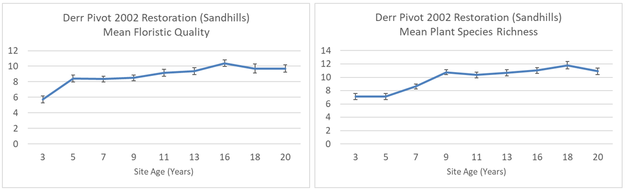
Since its third growing season (2004), I’ve been collecting plant community data from the site. Every other year, I go out with a 1x1m plot frame and list the plant species within 70-100 sampling plots scattered across the site in a stratified-random pattern (not permanent plots). From that, I can calculate both the species richness (number of species) and floristic quality of each square meter plot. Averaging those across the site gives me the mean species richness and mean floristic quality for that year.
(Reminder, if you want better views of graphs and photos, click on them. If you’re reading this within an email message, click on the post’s title to open it on the website and then clicking on images will work for you.)
Mean Floristic Quality (left) and Mean Species Richness (right) calculated from surveys of 70-100 1x1m quadrats. Both graphs seem to indicate a pretty rapid establishment of a plant community and then relative stability afterward. Error bars indicate 95% confidence intervals.
As you can see from the two graphs above, both the mean species richness and mean floristic quality increased during the first 8-10 years or so and then have leveled off. I’ve also found 143 plant species in those surveys, though that’s not a complete inventory of species, since those 1×1 plots don’t sample a very big percentage of the area each year.
That’s the boring background information. If you’re still with me, here’s where I’ll try to make it more interesting.
.
CHAPTER 1 – A PLANT COMMUNITY FORMS
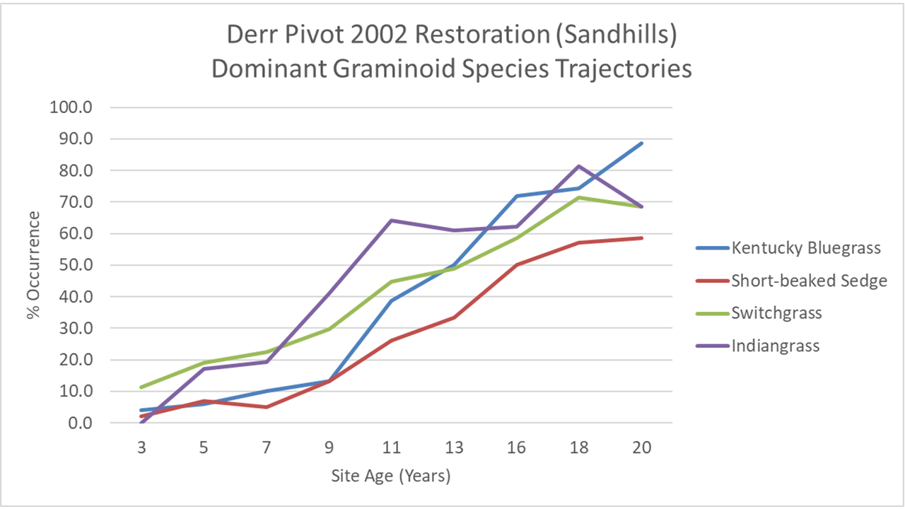
In addition to calculating richness and floristic quality metrics, I can also look at the frequency of occurrence of each species (the percent of 1×1 plots each species was found in) through the years. It doesn’t work well for plant species of low abundance, but for major grasses and forbs, I can look at how the abundance (essentially) of each species changed over time. Most of those species increased in occurrence over time and then leveled off. Others, like the three grasses and one sedge in the graph below, appear not to have hit their peak yet, even after 20 years.
Four surprisingly similar establishment trajectories for graminoids.
The graph shows the increasing frequency of occurrence of three grasses and one sedge (Carex brevior) over the first 20 years of this restored prairie’s life. Kentucky bluegrass wasn’t seeded, of course, and short-beaked sedge had a limited amount of seed, which helps explain why both started slowly. However, we had lots of switchgrass and Indiangrass seed, so why is it taking so long to fill in? That’s especially interesting because big bluestem – shown a few graphs below this – jumped out of the ground and was ubiquitous within a handful of years.
These graphs illustrate the assembly of a brand new prairie plant community over a 20 year period. Some species showed up in abundance within the first few years, but most started slowly and spread over time. The rate at which species increased in abundance to a point at which they seemed to reach their saturation point varied quite a bit.
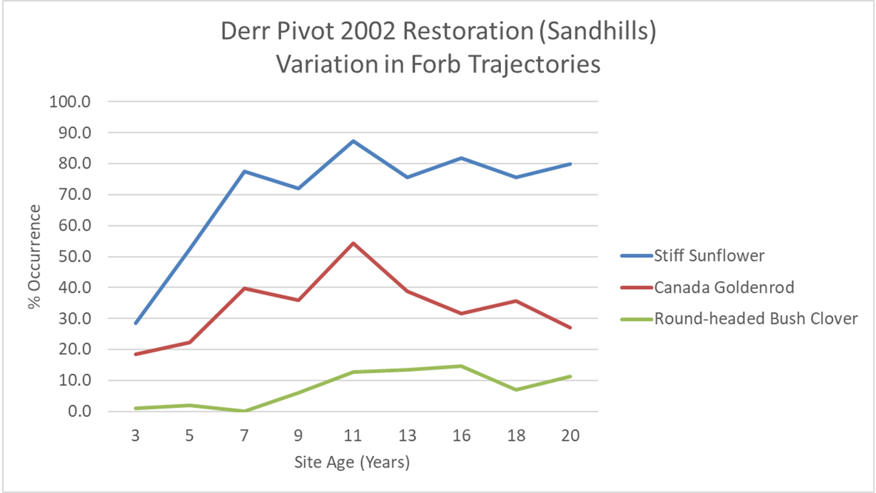
The graph below, for example, shows three very different patterns. Stiff sunflower (Helianthus pauciflorus) raced out to a fast start, and by year seven I was picking it up in 4 out 5 sampling plots. It has stayed roughtly at that level ever since. Canada goldenrod (Solidago canadensis) increased steadily until it was in half of my sampling plots in the 11th year of the planting, but then decreased just as steadily back to only 20% occurrence by year 20 – the same place it had been in year three. Round-headed bushclover (Lespedeza capitata), which is mostly found on hill tops and higher slopes, also took about 11 years to reach its peak, but, unlike the goldenrod, has maintained that level of abundance ever since.
Three very different patterns of establishment among common forb species in the restored prairie.This 2018 photo (year 17 of the prairie’s establishment) shows round-headed bushclover and stiff sunflower growing abundantly on a sandy hill top, surrounded by Junegrass, big bluestem, and many other plants. Each of those species followed its own path toward establishment in the community.
I mentioned big bluestem earlier. The graph below shows that big bluestem was already above 50% occurrence in the third year of the planting. That’s a significant difference from switchgrass, which was at 11% that year, and Indiangrass, which didn’t show up in any of my sampling plots at that stage. I don’t have an explanation for that, especially because harvested the grass seed myself with an old Massey combine, and while big bluestem was the most common of those three species in the sites I harvested, there was lots of Indiangrass and switchgrass too.
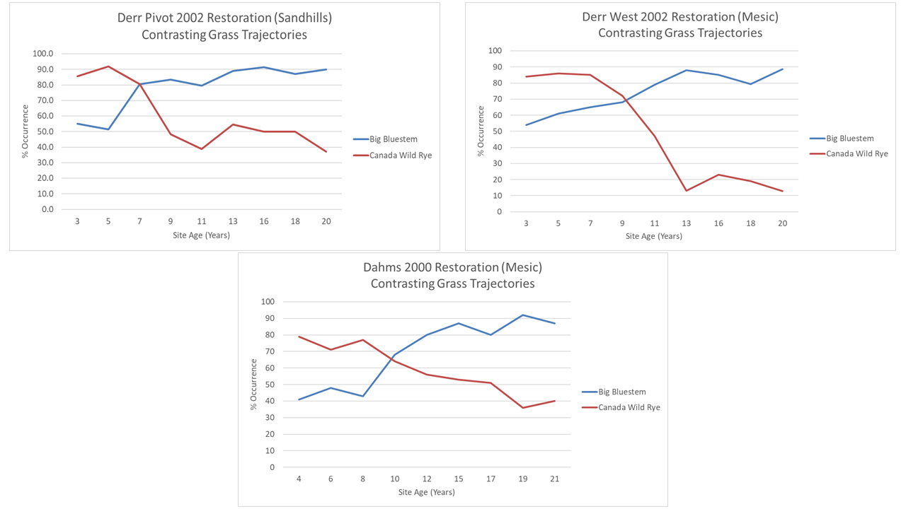
Canada wildrye and big bluestem show opposite patterns of abundance through time, though both were fast starters.
Even more fascinating to me, though, is the contrasting pattern of occurrence between big bluestem and Canada wildrye (Elymus canadensis). We worked hard to harvest lots of Canada wildrye seed because we know it tends to establish quickly but isn’t competitive against the other species we plant. That certainly held true here. It was at 86% occurrence at year three. But then, as big bluestem increased in abundance, Canada wildrye decreased, leveling out at 40-50% frequency of occurrence by year 9. It has held steady there since. I love being able to see evidence that supports the way I thought these two species worked in our plant communities. Big bluestem is a dominant force and Canada wildrye is more opportunistic, though both are perennial species.
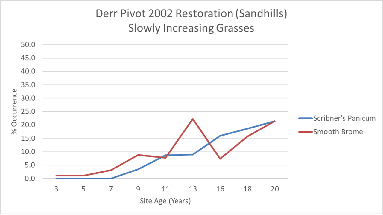
In contrast to big bluestem and Canada wildrye, two other grasses started out very slowly, and continue to increase very gradually. Scribner’s panicum (Panicum oligosanthes) is a great little native grass for which we had harvested very little seed. It’s not surprising, then, that it took a while to get going, and I’m encouraged that it continues to become more and more a part of the community. Smooth brome, on the other hand, can go jump in a lake as far as I’m concerned, but seems intent on slowly creeping in from the edges of the site. That could become a more significant issue over time if it suppresses plant diversity. So far, though, even at sites where it has already become much more widespread, our management seems to be keeping it from having a big effect on the community. We’ll see.
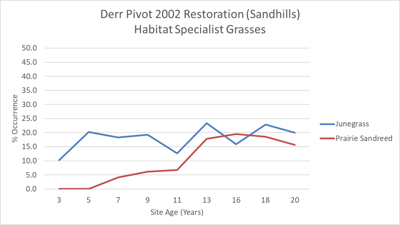
Finally, I wanted to talk about two grasses that are tied mostly to hill tops where the soil texture is most sandy. That restrictive habitat preference means they’ll be limited to a lower level of abundance than other species and both appear to have reached it. Junegrass (Koeleria macrantha), however, hit its plateau in year 5, while it took prairie sandreed (Calamovilfa longifolia) about 13 years to get to the same place (see graph below). I wouldn’t have guessed that, based on our seed harvest. We collected Junegrass by hand and didn’t have a particularly bounteous harvest, as I recall. I harvested prairie sandreed with our combine, and worked hard to get a lot of it, knowing it would do well in the sandhill habitat we were planting.
I think the explanation for Junegrass’ rapid rise is that it spread quickly by seed from its initial establishment points. It showed up right away from the seed we planted and then filled in the space around those first plants very quickly. Prairie sandreed, on the other hand, seemed to take a while to become full-size blooming plants, and appears to have spread primarily through rhizomes. Sandreed clones are now getting large (but are diffuse, not monocultures) and many are bigger than my kitchen. (You know my kitchen, right? The standard by which ecologists measure grass clones.)
Many species in the planting, including this shell leaf penstemon (Penstemon grandiflorus), are hugely variable in their abundance from year to year. It’s hard to pick up the patterns of that abundance with every-other-year sampling. This photo was taken in 2013, the year after the severe 2012 drought. The penstemon was one of a group of opportunists that thrived in that brief post-drought period of lower grass competition.
.
Ok, that’s Chapter 1. Compelling? No? Ok, give me a chance with Chapter 2 before you bail.
CHAPTER 2 – EVERY SITE IS DIFFERENT. MAYBE?
Having mined the data from the Derr Pivot site, I decided it would be interesting to compare the patterns of species establishment to that of other nearby plantings we’d done. I expected to see a lot of variation in those patterns because anyone who has done restoration work knows there’s a lot of unpredictability in that process. As it turned out, I found much more similarity than I’d expected.
I used two other restored prairies as comparisons. The first, the Derr West 2002 restoration was planted in the same year as the Derr Pivot, used seed from the same harvest effort, and is located a few hundred yards to the west. It had a more diverse seed mix because it was a more mesic site in alluvial soils, and we created some wetland sloughs that required appropriate seed. Basically, it received the same seed mix as the Derr Pivot site, but with the addition of wetland and wet-mesic species, bringing the species total in the mix to 218. I’ve been collecting data from Derr West every year since 2002, but am only showing data from every other year to match up with the Derr Pivot dataset.
The second site was planted two years earlier, and is called the Dahms 2000 planting. It is adjacent to the Derr West planting (just to the south), so all three of these sites are within the same square mile of land. The Dahms 2000 is also a mostly-mesic site on alluvial sandy loam soils, with some created wetland sloughs. The seed mix for it included 202 species. I collected data every other year from this site, but started doing so in alternating years to the Derr Pivot, so the time scale on the graphs doesn’t match perfectly.
Despite the similar geographic settings of all three, and the same seed mix (mostly) and establishment year for two of them, I expected to see a lot of variation in the rate at which individual species expressed themselves in community assembly. It’s fun to be wrong.
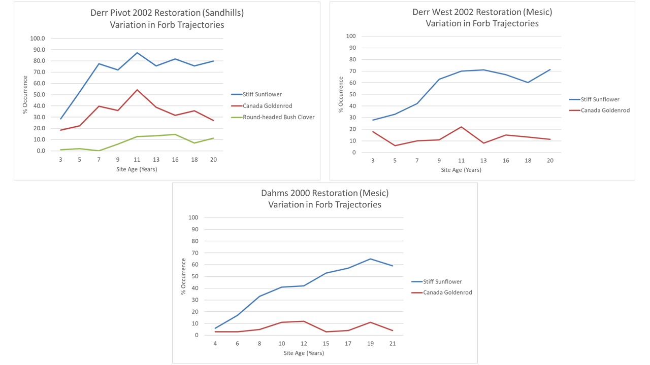
Let’s start with the three forbs I talked about earlier: stiff sunflower, Canada goldenrod, and round-headed bushclover. The two additional sites didn’t have enough abundance of the bush clover to track it, so I eliminated that one from the graphs below. But stiff sunflower and Canada goldenrod patterns were relatively similar between the three sites. They aren’t exact replicas, of course, but there’s more similarity than I’d expected.
Comparisons of stiff sunflower and Canada goldenrod establishment patterns across three sites.
Stiff sunflower took longer to hit its plateau in abundance at the second and third sites, compared to the Derr Pivot, but it still reached similar levels in all three plantings. We had a lot more seed for this species for the 2002 plantings than the 2000 planting, which might account for its faster start in those sites. Either way, though, the species worked its way into about 70-80% frequency of occurrence in all three plantings. Fascinating.
Canada goldenrod is much less abundant at both the additional sites, but in all three sites, its abundance is about the same in year 20 or 21 as it was in year 3 or 4. All three sites also appeared to see a bump in that abundance around 2012, though that may or may not be a real pattern. I know a lot of restoration sites have trouble with Canada goldenrod (or tall/late goldenrod, which in Nebraska is usually treated as a variety of Canada goldenrod). We seem to be fortunate here because Canada goldenrod doesn’t usually act aggressively in our plant communities.
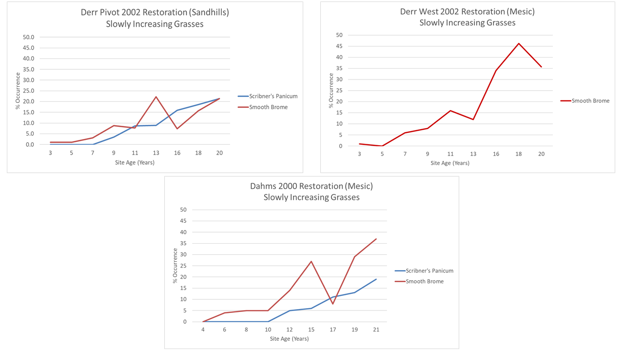
Next, let’s compare smooth brome and Scribner’s panicum, the two grasses that were slowly adding themselves to the community in the Derr Pivot. Scribner’s panicum is in the 2002 site, but at a low enough abundance that it isn’t yet able to be reliably tracked with my data collection method. In the Dahms 2000 restoration, though, it shows a remarkably similar pattern to that in the Derr Pivot, though it waited a little longer to show up in the data. I think we had even less seed for it in the 2000 planting than we did for the 2002 plantings, so that makes sense.
Scribner’s panicum (blue) and smooth brome (red) across three sites.
Smooth brome is also showing a very similar pattern of growth between the Derr Pivot and Dahms 2000 sites, including a temporary boost following the 2012 drought. The Derr West site shows a much faster establishment rate, but I can explain that. When that site was still a crop field, there was a weird peninsula of smooth brome and Siberian elm trees that extended into the field. When we prepared the site for restoration, we (I) did a poor job of killing those species out and during wetland construction, and brome sod got spread around the site, speeding its invasion. Sorry about that, everyone.
The similarities continue with big bluestem and Canada wildrye, which exhibit that same opposite pattern of establishment across all three sites. Canada wildrye ended up as a less significant player in the Derr West site than in the other two, but still followed the same kind of path to get there – starting high and the dropping low as the rest of the community filled in around it.
The final graph is the one that most surprised me. I just about fell out of my chair when I first put all three of these next to each other. I’ve spent my whole career being amazed by the complex and (to us) unpredictable nature of prairies and the restoration process. Now I look at these data and wonder if I’ve just been too dumb to notice patterns all around me.
For the record, I haven’t actually changed my mind about the complex and unpredictable nature of prairies. It is really neat, though, to discover some patterns in how things seem to work. I’d love to hear from other restoration sites about whether any data they might have line up with the patterns I’m seeing here. I also wish I’d had time to collect this kind of intensive data from more sites around here to see how consistent these patterns really are.
.
CHAPTER 3 – LAND STEWARDSHIP MATTERS, PEOPLE!
So, the story so far is that three prairies planted in the same area, within a few years of each other, showed remarkably similar patterns of plant community assembly over 20 years or so. All three of those sites have been managed with the same basic stewardship approach that combines prescribed fire and grazing. Patch-burn grazing is probably the best overall description of the approach, but it’s been modified to include periodic full seasons of rest from grazing.
Cattle grazing a recently burned patch of the Derr West restoration in 2021. The abundance of annual sunflowers are a response to the fire (triggers germination) but there are perennial sunflowers mixed in too.
While those three sites have been managed in basically the same way, we did build a nine acre exclosure in the Derr West restoration before we first grazed the site (in year 8 of its life). It receives the same frequency of burning (every 3-5 years) as the surrounding areas but isn’t grazed. It’s far from a perfect test or comparison (it’s not replicated and it’s in the corner of the larger site) but it does allow us a glimpse of how plant species might have established and acted if we were using fire but not grazing.
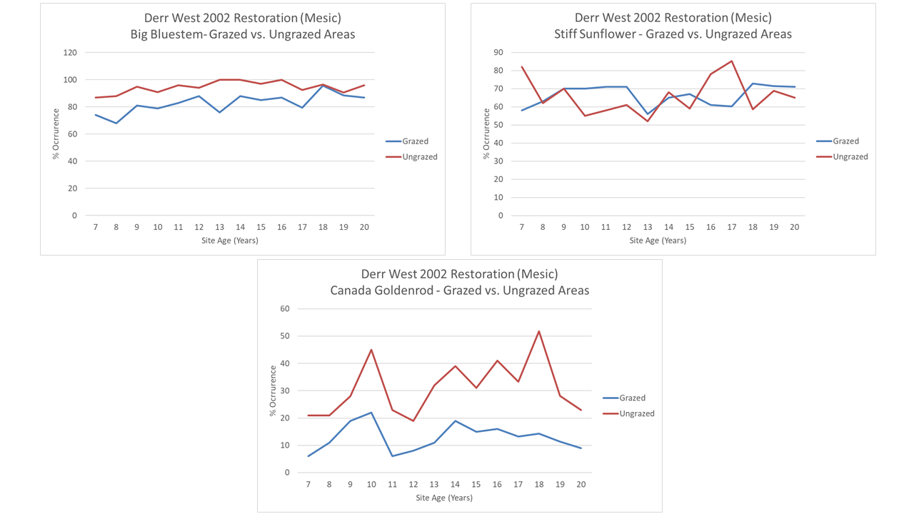
The following graphs illustrate the response of plants inside and outside of that exclosure at the Derr West restoration. I’m showing annual data here (not every other year) because I have it for this particular site. The first set of graphs below show three plant species for which grazing doesn’t seem to matter one way or the other. Big bluestem and stiff sunflower have maintained very steady patterns of abundance in both the grazed area and the exclosure. Canada goldenrod has a higher abundance in the ungrazed area, but that seems independent of grazing and the periodic ups and downs of its populations are nearly identical inside and outside of the grazing exclosure.
Big bluestem, stiff sunflower, and Canada goldenrod occurrence patterns with and without grazing at the Derr West restoration.
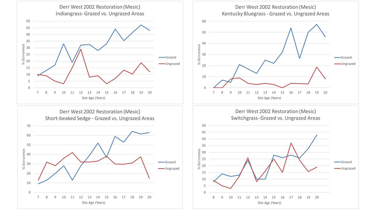
The story changes, though, when we look at the four graminoid species my previous graphs showed are steadily increasing at all three sites. Switchgrass looks like grazing doesn’t affect it much, but Indiangrass, Kentucky bluegrass, and the short-beaked sedge all seem to increase much faster under grazing. The results are pretty dramatic for Indiangrass and Kentucky bluegrass, in particular. If this is representative, the patterns of establishment for these species would have been very different if we’d not been grazing our sites during the later stages of their development. Since these graminoids are major components of the plant community, it’s intriguing to think about the ramifications of that.
Different reactions to grazing are apparent within these four graminoid species.
Finally, here are two examples of forbs that seem to show opposite reactions to grazing from each other. Maximilian sunflower (Helianthus maximiliani) has increased over time in the grazing exclosure, but has remained at a steady population level where it is being grazed. In contrast, upright prairie coneflower (Ratibida columnifera) has mostly disappeared from the exclosure, but is still around (more in some years than others) in the grazed part of the site.
Maximilian sunflower (left) and upright prairie coneflower (right) in grazed and ungrazed areas.
Comparing the broader plant communities between the grazed and ungrazed portions of the Derr West restoration is difficult because, again, the single grazing exclosure is in a corner of the larger site and doesn’t have the variation of soils found across the bigger ungrazed area. However, it is interesting to look at the trajectories of each since grazing first started in 2009 (second year of the graphs shown below).
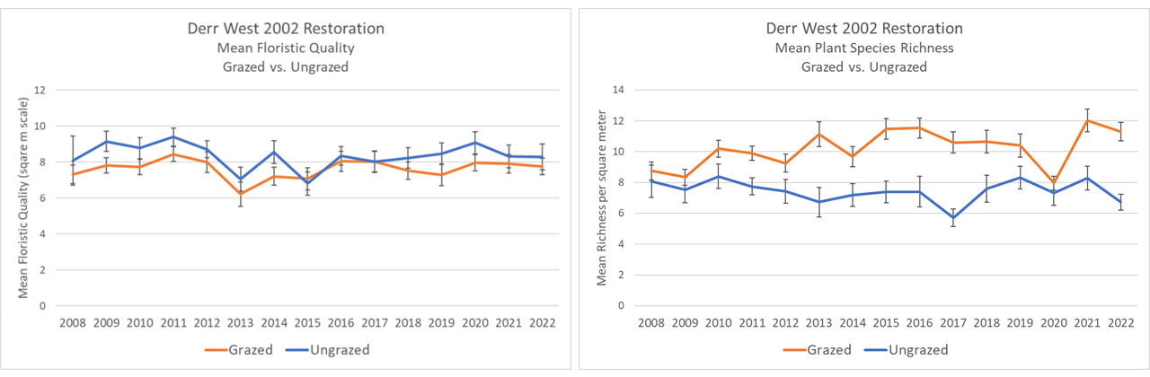
Mean floristic quality (left) and mean species richness (right) between the ungrazed exclosure (blue) and broader grazed site (red) at the Derr West 2002 Restoration. Error bars indicate 95% confidence intervals.
Mean floristic quality hasn’t really changed over time in either site. Mean species richness, however, has increased in the grazed area, gaining an average of 2 species per 1×1 meter plot over time (except in 2020 when excessive thatch suppressed growth). Does that make the grazed site better? Not necessarily, but the difference is intriguing.
Both the grazed and ungrazed areas still have diverse and interesting plant communities, but the management does affect both individual plant species and the broader community composition. In addition, of course, the grazing has big impacts on habitat structure, which is the primary reason we’re using it in the first place. There is a lot more habitat heterogeneity across the grazed site, providing for a more diverse animal community.
So, what can we draw from this long data-heavy post? During the community assembly stages of three restored plant communities, at least many of the major plant species followed remarkably similar trajectories of establishment. In some ways, that should be expected, given the similar sites, seed mixes, and weather patterns. On the other hand, anyone who has spent many years doing restoration work knows how variable results can be from year to year and site to site.
The species establishment trajectories at those three sites, however, seems to have been significantly influenced by management – at least for some species. If we can extrapolate from the grazing exclosure in the Derr West restoration, modified patch-burn grazing increased the establishment rate of some major grasses, but also the overall species richness (at the 1×1 meter scale).
This August 2015 photo shows the Derr Pivot restoration, full of stiff sunflower, prairie sand reed, and other plants. That plant community is still dynamic, with some species continuing to increase in abundance and others alternating between rare and abundant based on weather and management conditions.
The opportunity to watch plant communities emerge from bare ground and broadcast seed has been one of the most fascinating aspects of my career. We throw one seed mix across a large area and plant species sort themselves into communities that match soil and topography variation. Sometimes, that sorting process matches my expectations, but there are always surprises. Being able to go back and study that process via data helps me understand some of what I watched, but also introduces lots of new questions. I hope I get to watch these same sites for at least another 20 years or so because I don’t think the stories are going to get any less compelling.