Complications of Comparing Coefficients of Conservatism

Apologies for the nerdy subject matter in this post. I’m guessing it might be interesting to about 3% of you. For the rest of you, I tried to at least include a few pretty plant photos. I’ll try to write about something more universally interesting next time.

This is a post about the disparate ways coefficients of conservatism (C values) are assigned to plants in different places across the Central U.S. It’s not really a criticism of those variations, but more of a rumination about what those variations might tell us and a cautionary note about how to interpret floristic quality.

Lead plant and grazing cattle at the Niobrara Valley Preserve, Nebraska. This pasture is grazed every year, though at different times of the season, and receives periodic prescribed fire.

If you’re not familiar with C values, you can read more about them and floristic quality assessment (FQA) in this reprint of a 1997 publication that proposed FQA as a useful tool in Illinois. The 1997 publication by John Taft, Gerould Wilhelm, Doug Ladd, and Linda Masters built on from work by Floyd Swink and Gerould Wilhelm to build a floristic quality index. Taft et al. proposed FQA as a way to help assess “floristic integrity” or “floristic quality” in natural areas and to evaluate the effectiveness of stewardship work.

Floristic Quality Assessment has been much used and much criticized over the years. I am both a user and a critic. I appreciate it as a way to add some nuance/context to pure assessments of plant species richness (richness = the # of species present) and have applied it to some long-term monitoring efforts. In my monitoring data, though, I calculate floristic quality within a number of square meter quadrats and average those values across a site. As a result, I can look at change over time in both plant species richness and mean floristic quality (at the m2 scale) as two of many ways to evaluate a prairie and our stewardship efforts. (In case you’re wondering, the trends of the two metrics are nearly identical.)

One of my biggest concerns with FQA is that C values are assigned by botanists and there’s a lot of (necessary) subjectiveness in that process. That’s far from a unique take. However, I think the way plants are categorized highlight interesting regional/cultural differences about how we interpret “high-quality natural areas”, the effects of ecological disturbances, and how we define ecological degradation – and that’s actually what this post is about.

Dotted gayfeather has a c value of 5 in Kansas and Nebraska but is a 10 in Missouri and an 8 in Iowa.

If you look at the differences in the C values assigned to plant species in different states you can see what I mean. The figure below shows C values for nine plants and how broad the range of C values is between states (North and South Dakota have a combined list). These values are all publicly accessible, by the way, at universalfqa.org.

C values assigned by states (DAK = both South and North Dakota together) and the range of variation (right side) for each. Source: universalfqa.org

I’ll dive into those differences shortly. First, let’s look at the way C values are supposed to be assigned, based on the criteria in the Taft et al. publication linked above:

C value 0-1: Taxa adapted to severe disturbances, particularly anthropogenic disturbances, occurring so frequently that often only brief periods are available for growth and reproduction.

C value 2-3: Associated with somewhat more stable, though degraded, environments.

C values 4-6: These include many dominant or matrix species for several habitats; they have a high consistency of occurrence within given community types.

C values 7-8: Taxa we associate mostly with natural areas, but that can be found persisting where the habitat has been degraded somewhat.

C values 9-10: Restricted to high-quality natural areas.

Ok, now let’s consider the varying c values across states for the species listed above. Black-eyed Susan and sand dropseed are categorized by some states as, essentially, weeds that can grow anywhere there’s dirt (adapted to frequent severe disturbances). In others, they’re seen as “dominant or matrix species” and almost qualify as taxa associated “mostly with natural areas”. Is that because those two plants act differently in some states than others? Maybe. Or it could be that botanists are seeing them through very different lenses.

Black-eyed Susans in Nebraska seem to ebb and flow in abundance in response to surrounding plant competition.

Silver-leaf scurfpea and prairie violet are both easy to find at my family prairie. Most of that prairie was farmed until the early 1960s when it was planted back to (just) grasses. There are little patches of unplowed prairie scattered throughout, which lay unburned and surrounded by rowcrops for many years. After the farmed portions were planted to grass, the entire site was annually grazed, starting about 1964. That grazing wasn’t particularly conservation-focused until the last 20 years or so when I started to take over the management (which now has shifted to the open gate rotational grazing I’ve written about before).

Despite that, silver-leaf scurfpea and prairie violet are thriving at our family prairie (both are far more abundant than black-eyed Susan, interestingly). They did well in those unplowed, but grazed areas and have been moving into the adjacent grass plantings (scurfpea moved fast, violets are slower). Given that example (and I’ve seen both species in similar situations elsewhere in Nebraska) I’d argue they should both be given C values of 2 or 3 based on the above criteria. Nebraska, though, has them both at 6, which I guess I can live with, but Missouri gave the scurfpea a 9 and the violet a 10, meaning they are species found only in high quality natural areas.

Silver-leaf scurfpea seems very tolerant to relatively intense cattle grazing in Nebraska.

I want to be clear that I’m not saying the botanists that assigned these C values were dumb, or even wrong. Instead, I’m hoping to provoke some thought and discussion about this topic and point out that C values appear to be assigned very differently by different groups of botanists. That should give us great pause when trying to compare scores between states, including scores like mean C (average C value of the plants at a site) or FQA. In addition, even within a state, I think we should be looking closely and thinking carefully about how to interpret and use those scores.

Let’s see a couple more demonstrations of how differently C values are assigned between states. The graph below shows the percent of native plant species that are assigned a c value of 10 by different states across the Great Plains and Midwest.

Five states have assigned c values of 10 to 8% or less of their native plant species. Six states went the other way.

There seem to be two very different approaches – states that have given 1/5 to 1/4 of those native species a 10 and states that restrict that top value to 8% or less of those species. Why the stark difference in approach? It’s not really split between the Midwest and Great Plains, but I’m guessing it’s tied to local culture among botanists and conservationists in general.

As a final comparison, I graphed out the distribution of assigned C values across native plant species so we can compare two states – Indiana and Nebraska. Nebraska has a pretty regular bell curve to its distribution. Indiana does too, if you ignore the 24% of native species (!) with a C value of 10. It appears Nebraska considers a lot of their plants to be “matrix species” and Indiana has a lot of species they consider to be strongly tied to high quality natural areas.

Indiana and Nebraska look very different in terms of how C Values were assigned across native species. Source: universalfaq.org

I’m curious to hear what others think about this, but my suspicion is that botanists can slip into assigning values based on how easy it is to find certain plant species in the landscapes they know best. For example, soapweed/yucca is very common across much of Nebraska and Kansas, including in a lot of “degraded” prairies that have been chronically overgrazed. Cows don’t particularly like to eat it except during the winter or after a burn. So in Nebraska, it’s certainly not restricted to “high quality natural areas”. It is a species that can be difficult to eradicate – just ask some ranchers who have tried to do that.

Yucca (soapweed) in the Loess Hills of Iowa.

In Iowa and Missouri, the same yucca species is assigned a C value of 10. Is that because the kind of soil/topography conditions that favor yucca are really uncommon or because it has been extirpated from lots of sites because of poor management or other disturbances? In other words, is it sensitive to disturbances and missing from “degraded” sites? Or is it just rare because there aren’t many places with the topography and soils it needs? (These are earnest questions, by the way – I don’t know the answers.)

More to the point, the assignment of C values is based on some very loaded terminology. In particular, the words “anthropogenic disturbances”, “degraded” and “high quality” are prominent. In the paper by Taft and colleagues, there’s not much definition of either disturbance or degradation. It seems to be a “you know it when you see it” approach. That’s fine for people who see things the same way as the authors, but might be part of the reason we see such variation in c value assignment across different geographies.

Is grazing an automatic cause of degradation? By both cattle and bison? Are plants that thrive in frequently-grazed sites less conservative than those that thrive in ungrazed sites?

Also, of course, applying “anthropogenic disturbance” as a negative metric is super problematic – especially in Midwest and eastern Great Plains grasslands that originated and persist primarily because of people and their stewardship. In other words, “anthropogenic disturbance” is an integral part of those prairies, not an automatic cause of degradation. How do you think most of those fires happened prior to European colonization? (Spoiler: it wasn’t lightning.)

I could write a lot more about the conflicting and challenging criteria used to assign c values and the ways in which floristic quality can be used well and poorly, but most of that has already been covered very well by Greg Spyreas in an excellent overview. Instead, I’ll just say this: I worry that C values have sometimes been assigned to plants based, at least partly, on how excited a botanist would be to find them. We should keep that in mind as we interpret floristic quality scores.

Obviously, the way people feel about this topic and about the “quality” of habitats or species is related to how they view conservation success. Personally, I focus most on ecological resilience and how to grow and sustain that. Resilience is built on habitat size and species diversity. I’ve spent much of my career honing and popularizing restoration strategies that enlarge and reconnect habitat patches. I’ve also focused heavily on fire, grazing, and other stewardship practices that create habitat heterogeneity, and thus species diversity (of plants, animals, and other taxa).

While related, my focus is different from someone whose top priority is preventing rare species from going extinct. I don’t spend a lot of my time worrying about how to save any particular species. That’s not because I don’t care about them, but rather because I’m focused on the broader system that supports the long-term viability of all species.

Restored (replanted) prairie in Iowa, a state that has lost the vast majority of what many people would call “high quality prairie”, making it difficult to sustain populations of many prairie species without significant restoration efforts.

My particular attention toward resilience likely comes from the fact that I work mostly in Nebraska, where we still have a lot of prairie (about half of the state is in some kind of grassland cover). We have rare and at-risk species, but we also have a lot of prairie habitat to work with, especially compared to places like Illinois, for example, or some other states in the Midwest. That gives us a different perspective from each other, which understandably leads to different objectives and strategies.

And that brings us back to C values and how they’re assigned, used, and interpreted.

There are lots of people doing terrific conservation work, and among us, we represent a broad variety of perspectives and biases. Because of that, we vary in the way we view and measure conservation success. We also vary in the way we assign value to species and habitats. None of that is bad. It does, however, mean we shouldn’t work in silos.

I’ve learned a tremendous amount from site visits and/or discussions with friends and colleagues in all the states I’ve discussed here. Their perspectives have influenced mine, and I hope the reverse has been true as well. I think that assigning conservatism values to plant species can be a helpful way to interpret what we see in our respective prairies. Let’s just be careful not to rely on any single metric too much, especially metrics that are heavily influenced by cultural bias.

The Post-Grazing Year

At the beginning of the 2025 growing season, I picked out three sites I could visit repeatedly to photograph/document how a prairie responded to having been grazed the previous year. That turned out to be overly ambitious, but I did manage to focus on one of those sites – an 80×80 foot square marked out at our family prairie – and visited it frequently throughout 2025. I really enjoyed the project and happy to finally share a lot of my favorite photos from it.

One of the reasons I wanted to do this project is that many people have very limited experience with “conservation grazing”, or grazing that is aimed at achieving particular conservation objectives. That’s understandable if your only exposure to cattle grazing comes from seeing overgrazed pastures. As with most things, there’s a lot of variety out there. While it’s not hard to find examples of poorly-grazed grasslands across the Great Plains, there are also countless examples of very thoughtfully-applied grazing that create both good habitat for wildlife/pollinators/plant communities and profitability for ranchers. It’s important to highlight those examples and show that prairies can thrive under well-managed grazing.

Grazing has long been a significant component of prairie ecology. Today, it is still an important part of many prairies, particularly in the Great Plains. Grazing can be used to influence the competition between plants and determine the composition and diversity of the plant community. It can also shape habitat structure, creating areas of short, tall, and patchy vegetation, respectively. A mix of those various habitat types supports a diverse community of animals – large and small.

Here’s the plot on May 1. It was very short from being grazed the entire previous season. The yellower area in the top left is a different part of the same prairie that’s at a different stage of the grazing/rest cycle.

Much of the cattle grazing we’re experimenting with right now, both at The Nature Conservancy/Nebraska and at my family prairie, involves long periods of grazing followed by long periods of rest. There are lots of reasons for this approach, which I won’t go into here, but the biggest objective is to create a broad range of habitat structure across a prairie, without compromising the diversity and richness of the plant community. It’s about creating habitat heterogeneity and ecological resilience.

We’ve been managing our family prairie over the last 10-15 years with open-gate rotational grazing, which has a lot of similarities to patch-burn grazing but isn’t driven by fire. The 80×80 foot plot I photographed in 2025 had been grazed hard most of the previous season (June through October 2024) and part of the season before that (July through Mid-August 2023). By October 2024, it was uniformly short, with a fair amount of bare ground exposed (see the first photo of this post, which shows the plot at the beginning of the 2025 season).

This kind of grazing may sound (and look) irresponsible to people who are either uncomfortable with cattle grazing overall or who have been taught that you should never graze more than half of the biomass of a pasture before moving cattle out. An important point, though, is that the same pasture was rested for two full years prior to 2023/2024 and will be rested for two more full years before it is grazed again. That’s a lot of time for grazed plants to regain their energy and vigor. We’re also looking at how soils respond to this grazing pattern and are seeing positive results (more on that when the data is fully analyzed).

A big patch of purple prairie clover on June 27. Note how short the surrounding grasses are – they’re low on energy because of the previous year’s grazing. They’ll have recovered that energy by next year.
Stiff goldenrod was abundant and in full color on September 13. Again, note the sparsity and short height of the grasses and the space between plants.

My favorite part of grazing approaches like open-gate rotation and patch-burn grazing is the way the prairie community responds in the first year after a long season of grazing. The vigor of the typically-dominant plants (tall grasses, in particular) has been temporarily suppressed, releasing many other plants from that competitive pressure. This usually results in a big wildflower party, including both long-lived perennials and a lot of short-lived plants who are taking advantage of a short window of opportunity to germinate, bloom, and die while the big grasses aren’t able to prevent them from doing so.

The resulting habitat structure is terrific for many animal species, large and small. The reduced height and density of grasses means that it’s easy for animals to move through the vegetation. At the same time, other plants grow tall, creating a kind of miniature savanna, where tall wildflowers are like trees, surrounded by shorter vegetation. Animals can move from sun to shade easily to regulate their temperature. They can also can feed in open areas but quickly retreat to cover when they want to. This supports a huge abundance of invertebrates. It also draws in many larger animals, attracted both by the habitat structure and the food source (invertebrates).

In this October 7 photo, the foreground is the area featured in this post at the end of the 2025 growing season and the short-cropped area in the background is what was grazed hard in 2025 and will be rested in 2026 and 2027.

One highlight of the year was that I found purple coneflower in my plot (two different plants). I’ve only seen the species a few times during the 30 years or so I’ve been involved in the management of our family prairie and it had been a while since my last sighting. I wish I could tell you whether it was there because of some overseeding I did a few years ago or because it had been there a long time without me noticing it. Either way, it was really nice to find it.

Purple coneflower (Echinacea angustifolia)

Access to bare ground is crucial for many animals, including a lot of ground nesting bee species, bandwing grasshoppers, various invertebrate predators, and lots of others. Some of those need areas nearly free of any vegetation, but many just need places where the soil isn’t covered by a thick layer of thatch. Last year’s grazing removed most of the plant material from this part of the pasture and also tempered the growth of dominant grasses. The result was that there was lots of great habitat for species that need both bare soil and abundant sunlight.

The bare ground created by last year’s grazing made important habitat for lots of creatures, including this tiger beetle larva hunting at the top of its burrow.
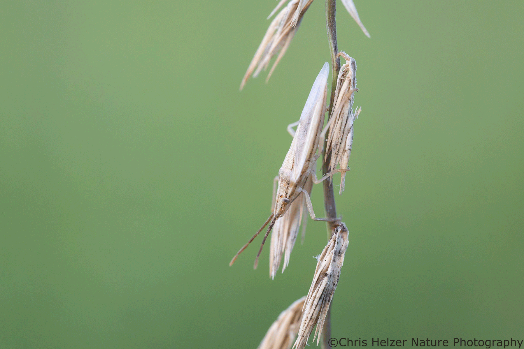
This narrow stink bug was well-camouflaged on its favorite food plant – sideoats grama.
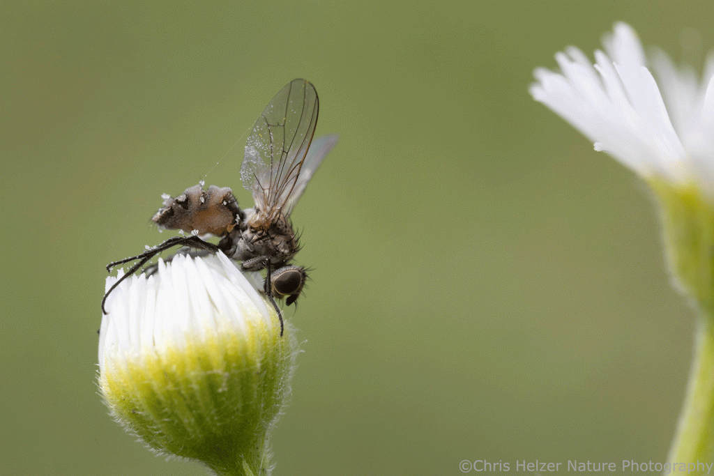
This fly was killed by a fungus that made it crawl to the top of this fleabane plant before dying. Read more about that here.
This bush katydid thought it was hiding from me by sitting still.

The following slideshows provide a visual journey through the 2024 season, from May through October. There are also two additional slideshows at the end, featuring lady beetles and crab spiders. If you’re reading this in an email, these slideshows will display as grids of images. If you click on the title of the post at the top of the email, you’ll be able to view this post online and will be able to scroll through the slideshow and see larger versions of the photos.

May Slideshow

June Slideshow

July/August Slideshow

September/October Slideshow

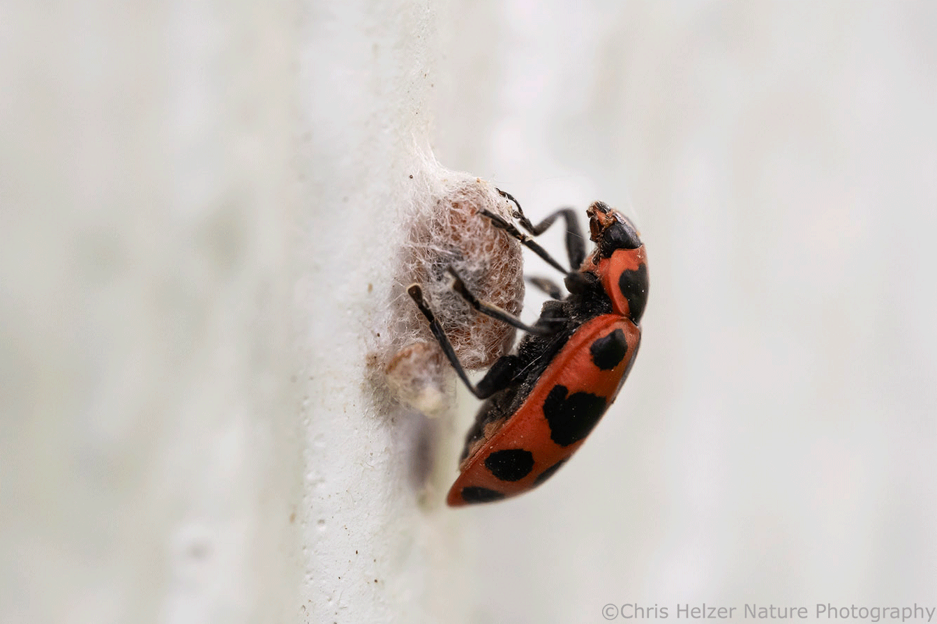
Finally, here are two last (short) slideshows featuring lady beetles and crab spiders. Why did I choose to highlight these two groups separately? That’s a great question. We all make decisions, don’t we?

Lady Beetles

Crab Spider Slideshow

For any of you who made it this far, I hope you enjoyed the results of this project. For me, it was a like a more relaxed version of my square meter project, in that I visited the same spot over and over through the season. An 80×80 foot plot seemed like a whole universe compared to that square meter, though.

Hopefully, the photos helped you visualize the ways in which a prairie can respond to cattle grazing. This single example, of course, shouldn’t be used to predict how other prairies might respond to similar management, though it was pretty typical of what I’ve seen on numerous sites in central Nebraska.

The most important message is that prairies have a lot of resilience built into them and it’s fascinating to watch that resilience on display. There are lots of good/right ways to manage prairies, depending upon your objectives, and we surely haven’t explored all of those yet. It’s ok to experiment with new approaches to see what happens. How else will we learn?